
The first part of the activity asks us to do get the Fourier transform on an aperture.

Figure1. On the left is the initial aperture, the fft2 transform of the aperture and on the right is the shifted fourier transform of the aperture
The first picture shows the initial aperture before the required transformation. The one on the middle on the other hand is the resulting image after the fft2 transformation of the aperture. It is interesting to see that indeed the fft2 transformation is inverted along its diagonal, just like what the AP186 manual said. The last picture shows the shifted transformation of the aperture. This, I think, is the required image, which is the real Fourier transform on the aperture.
 Figure2. Different apertures with their respective transforms on their side.
I also explored apertures with different sizes. Figure2 is a graphic (obviously) portrayal of my findings. As the aperture gets bigger, its transform seems to approach a dot. On the other hand, the transforms gets much more evident, and yes, eye-catching, if the aperture gets smaller. Also the transformation was done twice on the aperture, that is, after getting the Fourier transform of the aperture another Fourier transform was applied to the acquired transform. We found that applying the transform twice we got the same aperture back. Implying that we did nothing, or did we?
 Figure2. On the left an “A” aperture, its shifted fourier transform and the transform done twice on the aperture.
This time a big letter A was the object of our Fourier transform, this time the effect of applying the fft twice is very obvious. The image became inverted and the perfectly white area of A became blurred.
The second part of the activity involves convolution. Convolution is the smearing of one function to another. The resulting function is somewhat a combination of both. Say these two functions are f and g, their convolution will be given by ![]() Also this is also equivalent to
Also this is also equivalent to
 where H,F and G are the Fourier transform of h,f and g. Convolution is very useful since the concept is very much used in modeling optical systems. One such system is the lens system. Say f represents the object and g represents the transfer funcction of our lens. The convolution of f on g represents the image produced by the lens.
 Figure3. The VIP object
For this part, the convolution of the word VIP with two appertures was investigated. The resulting image is

Figure4. The apertures and the resulting convolution
As obviously seen the smaller aperture produced a very blurry image, even to the point of producing ripple-like patterns around the object. Meanwhile the larger aperture produced a better image. However, even with a larger aperture, the image produced did not really duplicate the original image. The VIP image produced has shadows or more like “penumbras” on the supposedly white areas of the original image. Also most obvious is the inversion of our image which is an expected behavior of our transform
The third part involves correlation. Correlation basically involves the degree of similarity between two functions f and g. Mathematically, ![]()
The correlation can also be given by  where P, F and G stands for the fourier transform of p, f, and g. The asterisk stands for complex conjugation of F and G.
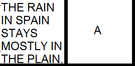
In this activity a sentence was correlated to a letter as shown by the images below

Figure5. The sentence and the letter that are to be correlated
From the definition of correlation, we expect to see something on the letters of A on the sentence. So without much further ado, the image will now be revealed..
.
.
.
.

Figure 6. The resulting correlation
The resulting image clearly shows the resulting correlation. So that something that we wanted to see are bright spots on the letter A. So we see that our correlation really worked, we sort of localized the A’s in our sentence as evidenced by the bright spots.
The last part is related to edged detection. Basically, I think this is just an extension of our correlation earlier. All we need is a mathematical representation of the edge we want to detect or emphasize. This can be done using the imcorrcoef() function in scilab. First, as stated above, we need the edges. Some representations are the following matrices.

Figure 7. The matrices representations of a horizontal, vertical, and spot edges
So let us look at the resulting images from the correlations

Figure 8. The matrices representations of a horizontal, vertical, and spot edges
The image a) used a horizontal template, curiously the horizontal edges were really emphasized and the vertical edges vanished. Image b on the other hand emphasized on the vertical lines so, now horizontal lines vanished. The third image used a spot template, so, this time, all lines were emphasized
Also on a side note, changing the magnitude of the matrix did not pose any noticeable change in the resulting image.
So for this activity, I will grade myself with 10.
I would like to thank Mr. Diaz, Mr. Abat for their insights and for helping me during those times I was lost
